design: dynamic kernel machine – dkm

Posted in AI/ML, Dave's Tools | Tagged | Leave a comment

dave’s random integer generator – drig

Project Name: drig
Destination: A Java Swing GUI application for demo random integer generation with given range and number requested – random lucky numbers generation for lottery.
Language: Java
IDE: NetBeans
Project Web: http://kenai.com/projects/drig
SVN address: https://svn.kenai.com/svn/drig~drig-src
Source Code: http://kenai.com/projects/drig/sources/drig-src/show
GUI Appearence:

Posted in Dave's Tools | Tagged , , , , , | 2 Comments

SVN quick guide for kenai project

A quick reference of svn on kenai project to submit, checkin and checkout source code as a dev. The intro focuses on Windows SVN with http/https and take ‘drig’ as an example. Great thanks to official help page: Using Subversion on Microsoft Windows Systems

1. Download SVN client from SourceForge: Win32 build for Subversion
2. Install SVN on your local machine
3. Access drig project source code on kenai: http://kenai.com/projects/drig/sources. Get address of SVN: https://svn.kenai.com/svn/drig~drig-src
4. Change directories to the location on your local machine where the repository will be checked out. For example:
 > cd myproj
5. Check out the server repository into a new directory. In the following command, Subversion creates the bluebird-svn directory for you.
 > svn co https://svn.kenai.com/svn/drig~drig-src
Note: Checking out the source for a project by using a URL like the one above pulls down all the branches and tags, in addition to the trunk code. If there’s already code in the repository, you might want to specify a subdirectory to select just the trunk or a branch or tag.
6. Copy a file to the local directory and then add it in subversion.
 > cp helloworld.java my_svn_dir
 > cd my_svn_dir
 > svn add helloworld.java
 > svn add *.java // batch operation
7. You see the following acknowledgment, which means that the file has been added and is ready to be checked in:
 A         helloworld.java
8. Update your local working copy (in case someone has checked files in while you were working):
 > svn update
9. Check the file into your project repository on the server:
 > svn commit helloworld.java -m”First commit to bluebird repository”
10. When prompted for your password, enter your project password. If the userid doesn’t match your password, you’re prompted for the project userid and then the password.
11. When the system accepts your entries, you see the following responses for the initial helloworld.java checkin:
 Adding         helloworld.java
 Transmitting file data.
 Committed revision 1.

Posted in Programming | Tagged , , | Leave a comment

time measurement for function call

Episode usage of ‘gettimeofday()’ and ‘times()

On Unix/Linux machine to measure the time consumption for certain function call, ‘gettimeofday’/’times’ would be 2 major ways. Better than ‘gettimeofday’, ‘times’ could provide detailed time info for user, system, child…

1. gettimeofday()

#include <sys/time.h>

struct timeval {
        long tv_sec;        /* seconds */
        long tv_usec;  /* microseconds */
};

struct timeval tpstart,tpend;
float timeuse = 0;
gettimeofday(&tpstart,NULL);
// function call
function_call();
gettimeofday(&tpend,NULL);
timeuse=1000000*(tpend.tv_sec-tpstart.tv_sec)+tpend.tv_usec-tpstart.tv_usec;
timeuse/=1000000;
printf(“Total time on function_call() is %fn”, timeuse);

2. times()

#include <sys/times.h>
#include <unistd.h>     // used by sysconf()

struct tms {
        clock_t tms_utime;  /* user time */
        clock_t tms_stime;  /* system time */
        clock_t tms_cutime; /* user time of children */
        clock_t tms_cstime; /* system time of children */
};

struct tms time_buf_head, time_buf_end;
long  tck = 0;
clock_t time_head, time_end;
tck = sysconf (_SC_CLK_TCK);
time_head = times( &time_buf_head );
// function call
function_call();
time_end = times( &time_buf_end );
printf(“function_call(), user time: %f, sys time: %f, child user time: %f, child sys time: %fn”,
        ((time_buf_end.tms_utime – time_buf_head.tms_utime) / (double)tck),
        ((time_buf_end.tms_stime – time_buf_head.tms_stime) / (double)tck),
        ((time_buf_end.tms_cutime – time_buf_head.tms_cutime) / (double)tck),
        ((time_buf_end.tms_cstime – time_buf_head.tms_cstime) / (double)tck) );

Posted in Programming | Tagged , , , , , | Leave a comment

kernel design approaches

A digest for kernel-wide design from wikipedia (including ALL the pics and some definitions)

1. Monolithic kernel (宏内核)

a: entire OS in kernel space and supervisor mode (eg, ring 0); b: a set of primitives or system calls for ALL OS services. E.g, BSD, Solaris, AIX, HP-UX, Linux, DOS, Window 9x

2. Microkernel (微内核)

a: near-minimum amount of OS – including address space management, thread management and IPC; b: device drivers, servers, protocol stacks, file systems, user interface, applications are ALL in user mode while kernel itself in supervisor mode or kernel mode; c: Microkernel servers are like daemon controlled by kernel. E.g, Mach, L4, QNX

3. Hybrid kernel (混内核)

a: kernel structure like microkernel, b: implemented like monolithic kernel, c: key OS services moved into kernel space while left (e.g, file systems) left in user space. E.g, Windows NT, BeOS, Plan 9, Inferno, NetWare

4. Nanokernel (纳内核, Picokernel)

a: much more small size from Microkernel, b: virtualization layer under OS – hypervisor, c: hardware abstraction layer at the bottom of OS.

5.  Exokernel (外内核)

a: the least abstraction of hardware – left to application good for distribute OS, b: library OS as middle ware between Application and kernel, c: end-to-end for application. E.g, Nemesis, ExOS.

Posted in OS | Tagged , , , , , , , | Leave a comment

trap – signal handling in shell

Ways for shell to create ‘multi-thread’ scripts (用shell写多线程脚本)

An enhancement for ‘tod‘(利用trap改进多线程shell脚本)

Yes, the way to write ‘multi-thread’ for shell is using ‘&’ to submit background job. We will use ‘tod’ for example: In ‘tod’, there are in total 3 shell scripts involved – main script ‘tod’, sub script ‘todss’ and sub script(cmd) ‘tcpdump’. Both ‘todss’ and ‘tcpdump’ are called in ‘tod’ as background job. The main purpose of ‘todss’ is to do detection of ‘tod’ to see if it is still alive or killed by user already. For the later case, ‘todss’ would kill the background ‘tcpdump’ and then exits. Now we are going to use ‘trap’ in ‘tod’ to implement signal handling – usually ^C. In this way, there is no need for use to implement ‘todss’ but only main script ‘tod’ and background ‘tcpdump’. Copy the episode of ‘tod’ here:

# Start main thread for ‘tod’
echo “tod: started”
touch $FILENAME
while true
do
        # daveti: Implement trap here to do signal handling
        # daveti: kill background ‘tcpdump’ and kill the shell itself
        trap “kill $TCPDUMP_PID; echo ‘tod: tcpdump killed’; echo ‘tod: exit’; kill $$” INT

        files=`ls $FILENAME* | wc -l`
        if [ “$files”  -gt 1 ]
        then
                # Only keep the 2 latest files on diskless
                for var in $(ls -t $FILENAME* | sed ‘1,2d’)
                do
                        scp $var $REMOTEMACH
                        rm $var
                done
        fi
        sleep 1
done

De facto, there are 3 different ways for ‘trap’: 1. trap “XXXX” signal-list – Catch the signals listed in ‘signal-list’ and do the corresponding actions ‘XXXX”; 2. trap “” signal-list – Ignore the signals in ‘signal-list’; 3. trap signal-list – Recover the default signal handling for signals in ‘signal-list’. Yes again, ‘trap’ could handle all the signals listed by ‘kill -l’ except ‘Signal 11’ – SIGSEGV. Also, to check the definition of certain signals in keyboard, use ‘stty -a’.

bash-2.05b$ kill -l
 1) SIGHUP       2) SIGINT       3) SIGQUIT      4) SIGILL
 5) SIGTRAP      6) SIGABRT      7) SIGBUS       8) SIGFPE
 9) SIGKILL     10) SIGUSR1     11) SIGSEGV     12) SIGUSR2
13) SIGPIPE     14) SIGALRM     15) SIGTERM     17) SIGCHLD
18) SIGCONT     19) SIGSTOP     20) SIGTSTP     21) SIGTTIN
22) SIGTTOU     23) SIGURG      24) SIGXCPU     25) SIGXFSZ
26) SIGVTALRM   27) SIGPROF     28) SIGWINCH    29) SIGIO
30) SIGPWR      31) SIGSYS      33) SIGRTMIN    34) SIGRTMIN+1
35) SIGRTMIN+2  36) SIGRTMIN+3  37) SIGRTMIN+4  38) SIGRTMIN+5
39) SIGRTMIN+6  40) SIGRTMIN+7  41) SIGRTMIN+8  42) SIGRTMIN+9
43) SIGRTMIN+10 44) SIGRTMIN+11 45) SIGRTMIN+12 46) SIGRTMIN+13
47) SIGRTMIN+14 48) SIGRTMIN+15 49) SIGRTMAX-15 50) SIGRTMAX-14
51) SIGRTMAX-13 52) SIGRTMAX-12 53) SIGRTMAX-11 54) SIGRTMAX-10
55) SIGRTMAX-9  56) SIGRTMAX-8  57) SIGRTMAX-7  58) SIGRTMAX-6
59) SIGRTMAX-5  60) SIGRTMAX-4  61) SIGRTMAX-3  62) SIGRTMAX-2
63) SIGRTMAX-1

bash-2.05b$ stty -a
speed 38400 baud; rows 40; columns 154; line = 0;
intr = ^C; quit = ^; erase = ^?; kill = ^U; eof = ^D; eol = <undef>; eol2 = <undef>; start = ^Q; stop = ^S; susp = ^Z; rprnt = ^R; werase = ^W;
lnext = ^V; flush = ^O; min = 1; time = 0;
-parenb -parodd cs8 -hupcl -cstopb cread -clocal -crtscts
-ignbrk -brkint -ignpar -parmrk -inpck -istrip -inlcr -igncr icrnl ixon -ixoff -iuclc -ixany -imaxbel
opost -olcuc -ocrnl onlcr -onocr -onlret -ofill -ofdel nl0 cr0 tab0 bs0 vt0 ff0
isig icanon iexten echo echoe echok -echonl -noflsh -xcase -tostop -echoprt echoctl echoke

Posted in Programming | Tagged , , , , , | 2 Comments

tcpdump on diskless – tod

Name: tod (无盘机器上的tcpdump)

Language: KSH

Destination: tcpdump on diskless

Orignal Intention: Run tcpdump on diskless machine where memory space is highly restricted

Version: 0.0

Supported Protocol: UDP/TCP/SCTP

Supported OS: Linux/FreeBSD/Solaris

Note: ‘root’ permission is preferred to avoid OS kernel error and ‘ssh’ key needs to be setup before running this tool

Example: ./tod -i bond0 -s 0 -w fpt06-s01c11h0_ngss -C 1 -p sctp -R root@172.96.64.152:/root/

P.S. ‘tod’ is written both for use and fun. Hope it useful for you.

Src:

#
# tcpdump on diskless – tod
# Version 0.0
# Oct 12, 2010
#
Dave.Tian@alcatel-lucent.com
#
# Changes:
# Limitation:
#       ‘tod’ is based on ‘tcpdump’ and ‘ssh’. Only 5 options from ‘tcpdump’ –
#       i, s, w, C, p – have been implemented in ‘tod’. For extra options support,
#       please modify ‘tod’ accordingly. For ‘ssh’ issue, ssh keys needs to be
#       constructed ahead of time to guarantee calling ‘scp’ without password.
#       ‘tod’ is NOT supporting multiple instance running on the same machine.
# Examples:
#       tod -i bond0 -s 0 -w fpt06-s01c11h0_ngss -C 1 -p sctp -R
root@172.96.64.152:/root/
#       tod -i eth0.400:4BAAA -s 0 -w tod_on_XXX -C 2 -R daveti@135.1.252.252/home/daveti/
#       tod -i eth0.400 -R root@172.96.64.152:/root/
#

# func:
show_usage() {
        echo “Usage: tod [-h] [-i <interface>] [-s <snaplen>] [-w <filename>] [-C <filesize>] [-p <protocol>] [-R <remoteMachine>]”
        echo ”  -h print this help message”
        echo ”  -p tcpdump option, protocol of the socket: udp/tcp/sctp”
        echo ”  -i tcpdump option, interface of the ethernet card”
        echo ”  -s tcpdump option, snaplen of the required packet, default value 0″
        echo ”  -w tcpdump option, file name for the tcpdump, default name ‘tod_dump'”
        echo ”  -C tcpdump option, file size limitation for each dump, default size 1(MB)”
        echo ”  -R scp option, remote machine to hold the dump from diskless (host IP is prefered), format:
login@IP:DIR
        echo “For detailed information about this tool, please refer to:”
        echo ” 
http://daveti.blog.com
        echo “Any feedback or suggestion please mail to:”
        echo ” 
Dave.Tian@alcatel-lucent.com
}

# Parameters’ processing for ‘tod’
typeset -i VAR_H
typeset -i VAR_I
typeset -i VAR_P
typeset -i VAR_S
typeset -i VAR_W
typeset -i VAR_C
typeset -i VAR_R
VAR_H=0
VAR_I=0
VAR_P=0
VAR_S=0
VAR_W=0
VAR_C=0
VAR_R=0
export INTERFACE=””
export PROTOCOL=””
export SNAPLEN=””
export FILENAME=””
export FILESIZE=””
export REMOTEMACH=””

 if [ “$#” != 0 ]
then
        while getopts hp:i:s:w:C:R: VAR
        do
                case $VAR in
                        h|H)
                                ((VAR_H+=1))
                                ;;
                        i|I)
                                ((VAR_I+=1))
                                INTERFACE=${OPTARG}
                                ;;
                        p|P)
                                ((VAR_P+=1))
                                PROTOCOL=${OPTARG}
                                ;;
                        s|S)
                                ((VAR_S+=1))
                                SNAPLEN=${OPTARG}
                                ;;
                        C|c)
                                ((VAR_C+=1))
                                FILESIZE=${OPTARG}
                                ;;
                        w|W)
                                ((VAR_W+=1))
                                FILENAME=${OPTARG}
                                ;;
                        R|r)
                                ((VAR_R+=1))
                                REMOTEMACH=${OPTARG}
                                ;;
                        ?)
                                show_usage
                                exit 1
                                ;;
                esac

        done

        shift $(($OPTIND – 1))
        VAR_R_ARG=”$*”

        if [ -n “$VAR_R_ARG” ] || [ “$VAR_I” = 0 ] || [ “$VAR_R” = 0 ] || [ “$VAR_H” = 1 ]
        then
                show_usage
                exit 1
        else
                if [ “$VAR_P” != 0 ] && [ “$PROTOCOL” != “udp” ] && [ “$PROTOCOL” != “tcp” ] && [ “$PROTOCOL” != “sctp” ]
                then
                        echo “Error: unsupported protocol. Only UDP/TCP/SCTP is supported by ‘tod'”
                        exit 1
                fi

                if [ “$VAR_S” = 0 ]
                then
                        echo “tod: Take default snaplen 0 for tcpdump”
                        SNAPLEN=”0″
                fi

                if [ “$VAR_C” = 0 ]
                then
                        echo “tod: Take default file size 1MB for tcpdump”
                        FILESIZE=”1″
                fi

                if [ “$VAR_W” = 0 ]
                then
                        echo “tod: Take default file name ‘tod_dump’ for tcpdump”
                        FILENAME=”tod_dump”
                fi
        fi
else
        show_usage
        exit 1
fi

# Construct ‘tcpdump’ cmd and get the PID
echo “tod: tcpdump started”
tcpdump -i $INTERFACE -s $SNAPLEN -w $FILENAME -C$FILESIZE -Z root $PROTOCOL &
TCPDUMP_PID=`ps | grep tcpdump | cut -d” ” -f1 | tr -d ” “`
if [ “$TCPDUMP_PID” = “” ]
then
        echo “Error: could not find the PID of tcpdump”
        echo “Warning: please kill the background job manually”
        exit 1
else
        echo “tod: PID of tcpdump: $TCPDUMP_PID”
fi

# Call for ‘todss’ with PID of ‘tod’ and PID of ‘tcpdump’
TOD_PID=`echo $$`
echo “tod: PID of todss: $TOD_PID”
if [ -f “$PWD/todss” ]
then
        echo “tod: todss started”
        ./todss $TOD_PID $TCPDUMP_PID &
else
        echo “Error: no ‘todss’ found in currrent directory”
        exit 1
fi

 # Start main thread for ‘tod’
echo “tod: started”
touch $FILENAME
while true
do
        files=`ls $FILENAME* | wc -l`
        if [ “$files”  -gt 1 ]
        then
                # Only keep the 2 latest files on diskless
                for var in $(ls -t $FILENAME* | sed ‘1,2d’)
                do
                        scp $var $REMOTEMACH
                        rm $var
                done
        fi
        sleep 1
done

#
# tcpdump on diskless sub script – todss
# Version 0.0
# Oct 12, 2010
#
Dave.Tian@alcatel-lucent.com
#
# Instruction:
#       This is a sub script called by ‘tod’. It acts as a sub thread
#       to detect if ‘tod’ is existed by ‘ctrl-c’ to determine if
#       background ‘tcpdump’ job is needed to be shutdown.
#

while true
do
        if [ “$(ps | grep ${1})” = “” ]
        then
                # Main ‘tod’ is exited; kill the ‘tcpdump’ job
                echo “todss: tcpdump stopped”
                # Note: only shell builtin kill accepts the job id as option,
                # however, seems builtin kill could not be called in script.
                # The possible reason should be independent job ids among
                # different sub shells. (That is why cmd kill works but script
                # kill complains: no such job.)
                # /bin/kill or /usr/bin/kill only accepts PID.
                # type -a kill: display the different kinds of kills.
                # So we will use PID instead of job id.
                kill ${2}
                exit 1
        else
                sleep 1
        fi
done


Posted in Dave's Tools | Tagged , , , , | 86 Comments

Jar usage

(1)Create jar (创建jar)
jar cf hello.jar hello 利用test目录生成hello.jar包,如hello.jar存在,则覆盖

(2)Create jar and display the process (创建并显示打包过程)
jar cvf hello.jar hello 利用hello目录创建hello.jar包,并显示创建过程
例:E:\>jar cvf hello.jar hello
标明清单(manifest)
增加:hello/(读入= 0) (写出= 0)(存储了 0%)
增加:hello/TestServlet2.class(读入= 1497) (写出= 818)(压缩了 45%)
增加:hello/HelloServlet.class(读入= 1344) (写出= 736)(压缩了 45%)
增加:hello/TestServlet1.class(读入= 2037) (写出= 1118)(压缩了 45%)

(3)Display Jar (显示jar包)
jar tvf hello.jar 查看hello.jar包的内容
指定的jar包必须真实存在,否则会发生FileNoutFoundException。

(4)Unzip jar (解压jar包)
jar xvf hello.jar 解压hello.jar至当前目录

(5)Add file into jar (jar中添加文件)
jar uf hello.jar HelloWorld.java 将HelloWorld.java添加到hello.jar包中

(6)Create jar without zipping (创建不压缩内容jar包)
jar cvf0 hello.jar *.class 利用当前目录中所有的.class文件生成一个不压缩jar包

(7)Create jar with manifest.mf (创建带manifest.mf文件的jar包)
jar cvfm hello.jar manifest.mf hello
创建的jar包多了一个META-INF目录,META-INF止录下多了一个manifest.mf文件,至于manifest.mf的作用,后面会提到.

(8)Create jar by ignoring manifest.mf (忽略manifest.mf文件)
jar cvfM hello.jar hello 生成的jar包中不包括META-INF目录及manifest.mf文件

(9)’-C’ usuage (加-C应用)
jar cvfm hello.jar mymanifest.mf -C hello/
表示在切换到hello目录下然后再执行jar命令

(10)Create index file with ‘-i’ (-i为jar文件生成索引列表)
当一个jar包中的内容很好的时候,你可以给它生成一个索引文件,这样看起来很省事。
jar i hello.jar 执行完这条命令后,它会在hello.jar包的META-INF文件夹下生成一个名为INDEX.LIST的索引文件,它会生成一个列表,最上边为jar包名。

(11)Redirect the process of unzipping (导出解压列表)
jar tvf hello.jar >hello.txt 如果你想查看解压一个jar的详细过程,而这个jar包又很大,屏幕信息会一闪而过,这时你可以把列表输出到一个文件中,慢慢欣赏!

(12)jar -cvf hello.jar hello/*
例如原目录结构如下:
hello
|—com
|—org

你本想只把com目录和org目录打包,而这时jar命令会连同hello目洋也一块打包进。这点大家要注意。jar命令生成的压缩文件会包含它后边出的 目录。我们应该进入到hello目录再执行jar命令。 注意:manifest.mf这个文件名,用户可以任指定,但jar命令只认识Manifest.mf,它会对用户指定的文件名进行相应在的转换,这不需 用户担心。

Posted in Programming | Tagged , | 2 Comments

Tune look&feel, language for NetBeans

To change the look&feel, language for NetBeans (改变NetBeans的外观和默认的语言环境), especially for the IDE on Windows XP with default language – Chinese: Modify ‘netbeans.conf’ under your ‘$NETBEANS_HOME/etc/’  by adding

–laf javax.swing.plaf.metal.MetalLookAndFeel //change the look&feel into Java metal style

–locale en_US // change the language into English, zh_CN is Chinese

# ${HOME} will be replaced by JVM user.home system property
netbeans_default_userdir=“${HOME}/.netbeans/6.7”

# Options used by NetBeans launcher by default, can be overridden by explicit
# command line switches:
netbeans_default_options=“-J-Dorg.glassfish.v3.installRoot=”C:Program Filessges-v3-prelude” -J-Dcom.sun.aas.installRoot=”C:SunAppServer” -J-client -J-Xss2m -J-Xms32m -J-XX:PermSize=32m -J-XX:MaxPermSize=200m -J-Xverify:none -J-Dapple.laf.useScreenMenuBar=true -J-Dsun.java2d.noddraw=true –laf javax.swing.plaf.metal.MetalLookAndFeel –locale en_US

# Note that a default -Xmx is selected for you automatically.
# You can find this value in var/log/messages.log file in your userdir.
# The automatically selected value can be overridden by specifying -J-Xmx here
# or on the command line.

# If you specify the heap size (-Xmx) explicitely, you may also want to enable
# Concurrent Mark & Sweep garbage collector. In such case add the following
# options to the netbeans_default_options:
# -J-XX:+UseConcMarkSweepGC -J-XX:+CMSClassUnloadingEnabled -J-XX:+CMSPermGenSweepingEnabled
# (see
http://wiki.netbeans.org/wiki/view/FaqGCPauses)

# Default location of JDK, can be overridden by using –jdkhome <dir>:
netbeans_jdkhome=“D:programJavajdk1.6.0_16”

# Additional module clusters, using ${path.separator} (‘;’ on Windows or ‘:’ on Unix):
#netbeans_extraclusters=”/absolute/path/to/cluster1:/absolute/path/to/cluster2″

# If you have some problems with detect of proxy settings, you may want to enable
# detect the proxy settings provided by JDK5 or higher.
# In such case add -J-Djava.net.useSystemProxies=true to the netbeans_default_options.

Posted in IDE_Make | Tagged , | 4 Comments

Kernel Functions in Machine Learning (Transfered)

Kernel Functions for Machine Learning Applications

Published Wednesday, March 17, 2010 by César Souza in , ,

In recent years, Kernel methods have received major attention, particularly due to the increased popularity of the Support Vector Machines. Kernel functions can be used in many applications as they provide a simple bridge from linearity to non-linearity for algorithms which can be expressed in terms of dot products. In this article, we will list a few kernel functions and some of their properties.

Many of these functions have been incorporated in Accord.NET, a extension framework for the popular AForge.NET Framework which also includes many other statistics and machine learning tools.

Contents

  1. Kernel Methods
    1. The Kernel Trick
    2. Kernel Properties
    3. Choosing the Right Kernel
  2. Kernel Functions
    1. Linear Kernel
    2. Polynomial Kernel
    3. Gaussian Kernel
    4. Exponential Kernel
    5. Laplacian Kernel
    6. ANOVA Kernel
    7. Hyperbolic Tangent (Sigmoid) Kernel
    8. Rational Quadratic Kernel
    9. Multiquadric Kernel
    10. Inverse Multiquadric Kernel
    11. Circular Kernel
    12. Spherical Kernel
    13. Wave Kernel
    14. Power Kernel
    15. Log Kernel
    16. Spline Kernel
    17. B-Spline Kernel
    18. Bessel Kernel
    19. Cauchy Kernel
    20. Chi-Square Kernel
    21. Histogram Intersection Kernel
    22. Generalized Histogram Intersection Kernel
    23. Generalized T-Student Kernel
    24. Bayesian Kernel
    25. Wavelet Kernel
  3. Source Code
  4. See Also
  5. References


Kernel Methods

Kernel methods are a class of algorithms for pattern analysis, whose best known element is the support vector machine (SVM). The general task of pattern analysis is to find and study general types of relations (for example clusters, rankings, principal components, correlations, classifications) in general types of data (such as sequences, text documents, sets of points, vectors, images, etc).

KMs approach the problem by mapping the data into a high dimensional feature space, where each coordinate corresponds to one feature of the data items, effectively transforming the data into a set of points in a Euclidean space. In that space, a variety of methods can be used to find relations in the data. Since the mapping can be quite general (not necessarily linear, for example), the relations found in this way are accordingly very general. This mapping approach is called the kernel trick.

The Kernel Trick

The kernel trick can be applied to any algorithm that solely depends on the dot product between two vectors. Wherever a dot product is used, it is replaced by a kernel function. When done, linear algorithms are transformed into a non-linear algorithms. Those non-linear algorithms are equivalent to their linear originals operating in the range space of a feature space φ. However, because kernels are used, the φ function does not need to be ever explicitly computed. This is highly desirable, as sometimes our higher-dimensional feature space could even be infinite-dimensional and thus infeasible to compute.

Kernel Properties

Kernel functions must be continuous, symmetric, and most preferably should have a positive (semi-)definite Gram matrix. Kernels which are said to satisfy the Mercer’s theorem are positive semi-definite, meaning their kernel matrices have no non-negative Eigen values. The use of a positive definite kernel insures that the optimization problem will be convex and solution will be unique.

However, many kernel functions which aren’t strictly positive definite also have been shown to perform very well in practice. An example is the Sigmoid kernel, which, despite its wide use, it is not positive semi-definite for certain values of its parameters. Boughorbel (2005) also experimentally demonstrated that Kernels which are only conditionally positive definite can possibly outperform most classical kernels in some applications.

Kernels also can be classified as anisotropic stationary, isotropic stationary, compactly supported, locally stationary, nonstationary or separable nonstationary. Moreover, kernels can also be labeled scale-invariant or scale-dependant, which is an interesting property as scale-invariant kernels drive the training process invariant to a scaling of the data.

Choosing the Right Kernel

Choosing the most appropriate kernel highly depends on the problem at hand – and fine tuning its parameters can easily become a tedious and cumbersome task. Automatic kernel selection is possible and is discussed in the works by Tom Howley and Michael Madden.

The choice of a Kernel depends on the problem at hand because it depends on what we are trying to model. A polynomial kernel, for example, allows us to model feature conjunctions up to the order of the polynomial. Radial basis functions allows to pick out circles (or hyperspheres) – in constrast with the Linear kernel, which allows only to pick out lines (or hyperplanes).

The motivation behind the choice of a particular kernel can be very intuitive and straightforward depending on what kind of information we are expecting to extract about the data. Please see the final notes on this topic from Introduction to Information Retrieval, by Manning, Raghavan and Schütze for a better explanation on the subject.

Kernel Functions

Below is a list of some kernel functions available from the existing literature. As was the case with previous articles, every LaTeX notation for the formulas below are readily available from their alternate text html tag. I can not guarantee all of them are perfectly correct, thus use them at your own risk. Most of them have links to articles where they have been originally used or proposed.

1. Linear Kernel

The Linear kernel is the simplest kernel function. It is given by the inner product <x,y> plus an optional constant c. Kernel algorithms using a linear kernel are often equivalent to their non-kernel counterparts, i.e. KPCA with linear kernel is the same as standard PCA.

k(x, y) = x^T y + c

2. Polynomial Kernel

The Polynomial kernel is a non-stationary kernel. Polynomial kernels are well suited for problems where all the training data is normalized.

k(x, y) = (alpha x^T y + c)^d  
Adjustable parameters are the slope alpha, the constant term c and the polynomial degree d.

3. Gaussian Kernel

The Gaussian kernel is an example of radial basis function kernel.

k(x, y) = expleft(-frac{ lVert x-y rVert ^2}{2sigma^2}right)

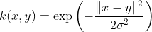
Alternatively, it could also be implemented using

k(x, y) = expleft(- gamma lVert x-y rVert ^2 )

The adjustable parameter sigma plays a major role in the performance of the kernel, and should be carefully tuned to the problem at hand. If overestimated, the exponential will behave almost linearly and the higher-dimensional projection will start to lose its non-linear power. In the other hand, if underestimated, the function will lack regularization and the decision boundary will be highly sensitive to noise in training data.

4. Exponential Kernel

The exponential kernel is closely related to the Gaussian kernel, with only the square of the norm left out. It is also a radial basis function kernel.

k(x, y) = expleft(-frac{ lVert x-y rVert }{2sigma^2}right)

5. Laplacian Kernel

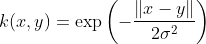
The Laplace Kernel is completely equivalent to the exponential kernel, except for being less sensitive for changes in the sigma parameter. Being equivalent, it is also a radial basis function kernel.

k(x, y) = expleft(- frac{lVert x-y rVert }{sigma}right)

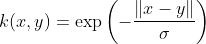
It is important to note that the observations made about the sigma parameter for the Gaussian kernel also apply to the Exponential and Laplacian kernels.

6. ANOVA Kernel

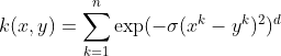
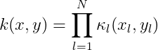
The ANOVA kernel is also a radial basis function kernel, just as the Gaussian and Laplacian kernels. It is said to perform well in multidimensional regression problems (Hofmann, 2008).

k(x, y) =  sum_{k=1}^n  exp (-sigma (x^k - y^k)^2)^d

7. Hyperbolic Tangent (Sigmoid) Kernel

The Hyperbolic Tangent Kernel is also known as the Sigmoid Kernel and as the Multilayer Perceptron (MLP) kernel. The Sigmoid Kernel comes from the Neural Networks field, where the bipolar sigmoid function is often used as an activation function for artificial neurons.

k(x, y) = tanh (alpha x^T y + c)

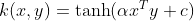
It is interesting to note that a SVM model using a sigmoid kernel function is equivalent to a two-layer, perceptron neural network. This kernel was quite popular for support vector machines due to its origin from neural network theory. Also, despite being only conditionally positive definite, it has been found to perform well in practice.

There are two adjustable parameters in the sigmoid kernel, the slope alpha and the intercept constant c. A common value for alpha is 1/N, where N is the data dimension. A more detailed study on sigmoid kernels can be found in the works by Hsuan-Tien and Chih-Jen.

8. Rational Quadratic Kernel

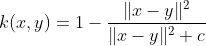
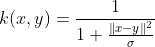
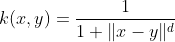
The Rational Quadratic kernel is less computationally intensive than the Gaussian kernel and can be used as an alternative when using the Gaussian becomes too expensive.

k(x, y) = 1 - frac{lVert x-y rVert^2}{lVert x-y rVert^2 + c}

9. Multiquadric Kernel

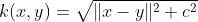
The Multiquadric kernel can be used in the same situations as the Rational Quadratic kernel. As is the case with the Sigmoid kernel, it is also an example of an non-positive definite kernel.

 k(x, y) = sqrt{lVert x-y rVert^2 + c^2}

10. Inverse Multiquadric Kernel

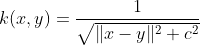
The Inverse Multi Quadric kernel. As with the Gaussian kernel, it results in a kernel matrix with full rank (Micchelli, 1986) and thus forms a infinite dimension feature space.

k(x, y) = frac{1}{sqrt{lVert x-y rVert^2 + theta^2}}

11. Circular Kernel

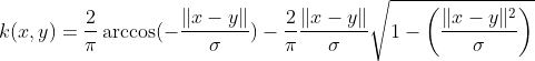
The circular kernel comes from a statistics perspective. It is an example of an isotropic stationary kernel and is positive definite in R2.

k(x, y) = frac{2}{pi} arccos ( - frac{ lVert x-y rVert}{sigma}) - frac{2}{pi} frac{ lVert x-y rVert}{sigma} sqrt{1 - left(frac{ lVert x-y rVert^2}{sigma} right)}
mbox{if}~ lVert x-y rVert < sigma mbox{, zero otherwise}

12. Spherical Kernel

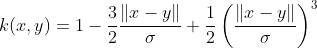
The spherical kernel is similar to the circular kernel, but is positive definite in R3.

k(x, y) = 1 - frac{3}{2} frac{lVert x-y rVert}{sigma} + frac{1}{2} left( frac{ lVert x-y rVert}{sigma} right)^3

mbox{if}~ lVert x-y rVert < sigma mbox{, zero otherwise}

13. Wave Kernel

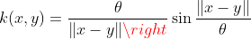
The Wave kernel is also symmetric positive semi-definite (Huang, 2008).

k(x, y) = frac{theta}{lVert x-y rVert right} sin frac{lVert x-y rVert }{theta}

14. Power Kernel

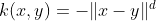
The Power kernel is also known as the (unrectified) triangular kernel. It is an example of scale-invariant kernel (Sahbi and Fleuret, 2004) and is also only conditionally positive definite.

k(x,y) = - lVert x-y rVert ^d

15. Log Kernel

The Log kernel seems to be particularly interesting for images, but is only conditionally positive definite.

k(x,y) = - log (lVert x-y rVert ^d + 1)

16. Spline Kernel

The Spline kernel is given as a piece-wise cubic polynomial, as derived in the works by Gunn (1998).

k(x, y) = 1 + xy + xy~min(x,y) - frac{x+y}{2}~min(x,y)^2+frac{1}{3}min(x,y)^3

However, what it actually mean is:

k(x,y) = prod_{i=1}^d 1 + x_i y_i + x_i y_i min(x_i, y_i) - frac{x_i + y_i}{2} min(x_i,y_i)^2 + frac{min(x_i,y_i)^3}{3}

Withx,y in R^d

17. B-Spline (Radial Basis Function) Kernel

The B-Spline kernel is defined on the interval [−1, 1]. It is given by the recursive formula:

k(x,y) = B_{2p+1}(x-y)

mbox{where~} p in N mbox{~with~} B_{i+1} := B_i otimes  B_0.

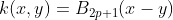
In the work by Bart Hamers it is given by:k(x, y) = prod_{p=1}^d B_{2n+1}(x_p - y_p)

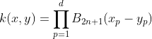
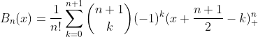
Alternatively, Bn can be computed using the explicit expression (Fomel, 2000):

B_n(x) = frac{1}{n!} sum_{k=0}^{n+1} binom{n+1}{k} (-1)^k (x + frac{n+1}{2} - k)^n_+

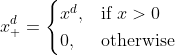
Where x+ is defined as the truncated power function:

 x^d_+ = begin{cases} x^d, & mbox{if }x > 0 \  0, & mbox{otherwise} end{cases}

18. Bessel Kernel

The Bessel kernel is well known in the theory of function spaces of fractional smoothness. It is given by:

k(x, y) = frac{J_{v+1}( sigma lVert x-y rVert)}{ lVert x-y rVert ^ {-n(v+1)} }

where J is the Bessel function of first kind. However, in the Kernlab for R documentation, the Bessel kernel is said to be:

k(x,x') = - Bessel_{(nu+1)}^n (sigma |x - x'|^2)

19. Cauchy Kernel

The Cauchy kernel comes from the Cauchy distribution (Basak, 2008). It is a long-tailed kernel and can be used to give long-range influence and sensitivity over the high dimension space.

k(x, y) = frac{1}{1 + frac{lVert x-y rVert^2}{sigma} }

20. Chi-Square Kernel

The Chi-Square kernel comes from the Chi-Square distribution.

k(x,y) = 1 - sum_{i=1}^n frac{(x_i-y_i)^2}{frac{1}{2}(x_i+y_i)}

21. Histogram Intersection Kernel

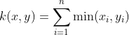
The Histogram Intersection Kernel is also known as the Min Kernel and has been proven useful in image classification.

k(x,y) = sum_{i=1}^n min(x_i,y_i)

22. Generalized Histogram Intersection

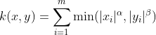
The Generalized Histogram Intersection kernel is built based on the Histogram Intersection Kernel for image classification but applies in a much larger variety of contexts (Boughorbel, 2005). It is given by:

k(x,y) = sum_{i=1}^m min(|x_i|^alpha,|y_i|^beta)

23. Generalized T-Student Kernel

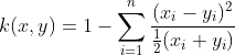
The Generalized T-Student Kernel has been proven to be a Mercel Kernel, thus having a positive semi-definite Kernel matrix (Boughorbel, 2004). It is given by:

k(x,y) = frac{1}{1 + lVert x-y rVert ^d}

24. Bayesian Kernel

The Bayesian kernel could be given as:

k(x,y) = prod_{l=1}^N kappa_l (x_l,y_l)where

kappa_l(a,b) = sum_{c in {0;1}} P(Y=c mid X_l=a) ~ P(Y=c mid X_l=b)

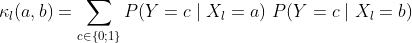
However, it really depends on the problem being modeled. For more information, please see the work by Alashwal, Deris and Othman, in which they used a SVM with Bayesian kernels in the prediction of protein-protein interactions.

25. Wavelet Kernel

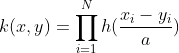
The Wavelet kernel (Zhang et al, 2004) comes from Wavelet theory and is given as:

k(x,y) = prod_{i=1}^N h(frac{x_i-c_i}{a}) :  h(frac{y_i-c_i}{a})
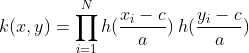
Where a and c are the wavelet dilation and translation coefficients, respectively (the form presented above is a simplification, please see the original paper for details). A translation-invariant version of this kernel can be given as:

k(x,y) = prod_{i=1}^N h(frac{x_i-y_i}{a})
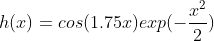
Where in both h(x) denotes a mother wavelet function. In the paper by Li Zhang, Weida Zhou, and Licheng Jiao, the authors suggests a possible h(x) as:

h(x) = cos(1.75x)exp(-frac{x^2}{2})Which they also prove as an admissible kernel function.

Source Code

The latest version of the source code for some of the kernels listed above is available in the Accord.NET Framework. Some are also available in the sequel of this article, Kernel Support Vector Machines for Classification and Regression in C#. They are provided together with a comprehensive and simple implementation of SVMs (Support Vector Machines) in C#. However, for the latest sources, which may contain bug fixes and other enhancements, please download the most recent version available of Accord.NET.

See also


References

Citing this work

If you would like, please cite this work as: Souza, César R. “Kernel Functions for Machine Learning Applications.” 17 Mar. 2010. Web. <http://crsouza.blogspot.com/2010/03/kernel-functions-for-machine-learning.html&gt;.

Posted in AI/ML | Tagged , , | 6 Comments